Predicting long-time dynamics from short-time information is a promising way of studying how equilibrium is approached for an open quantum system starting from a non-equilibrium initial condition.
This post discusses one of the prediction methods for long-time open system dynamics, the transfer tensor method (TTM)[1]. The TTM is based on, (i) the Nakajima-Zwanzig equation equation of an open quantum system Eq. \eqref{eq:1}, and (ii) the assumption that the state of the open system at time $t$ is barely correlated with the state at $t’$ if $|t-t’|$ is greater than a certain threshold. Let’s start from the Nakajima-Zwanzig equation of an open system[2]:
where $\mathcal{L}_{s}$ is the Liouville operator corresponding to the system part of the system-bath Hamiltonian, and $\rho(t)$ is the system reduced density matrix. The memory kernel $\mathcal{K}(\tau)$ measures how correlated a state $\rho(t)$ is to a previous state $\rho(t-\tau)$. This this equation can be discretized on time grids $(0, \delta, 2\delta, \ldots, N\delta)$ as follows (superscripts below are the time grids: $\mathcal{K}_{n}=\mathcal{K}({n\delta})$ and such):
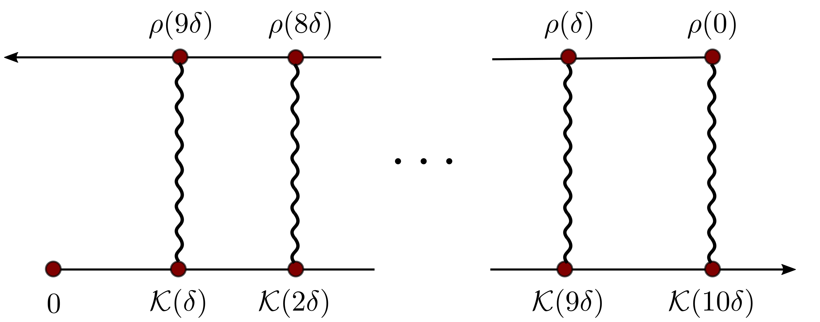
This means, if we know that memory kernel $\mathcal{K}(t)$ decays to zero after a certain time $t_\mathrm{max}$, we can use the memory kernel and reduced density matrices before $t_\mathrm{max}$ to calculate the reduced density matrix to as long a time as we want. For example, if $\mathcal{K}(t>10\delta)=0$, we can use a sequence of initial density matrices $\rho_0,\ldots,\rho_{9}$ and $\mathcal{K}_{1},\ldots,\mathcal{K}_{10}$ to calculate ${\rho}_{10}$. Again, based on ${\rho_{1}},\ldots,{\rho_{11}}$ (just obtained in the last step) and $\mathcal{K}_{1},\ldots,\mathcal{K}_{10}$ we can obtain ${\rho}_{11}$. This calculation can go on and on until we get the density matrix at a desired long enough time.
The question is how to obtain the initial sequence ${\rho_{1}},\ldots,{\rho_{10}}$ and $\mathcal{K}_{1},\ldots,\mathcal{K}_{10}$. The density matrix part can be easily obtained by simulating the open system with an desired initial condition. The memory kernel is a bit more difficult to obtain. To calculate $\mathcal{K}_n$, we first note that Eq. \eqref{eq:2} can be rewritten as
where we define the Liouville space matrix that maps $\rho_0$ to $\rho_N$ to be $\mathcal{E}_N$ and $\mathcal{E}_0=1$. This matrix doesn’t depend on the initial state $\rho_0$ (e.g. $\mathcal{E}_1=1- \frac{i}{\hbar} \mathcal{L}_{s} - \mathcal{K}_1$). If $\mathcal{E}_n$ can be obtained, the memory kernels can be solved for iteratively:
\begin{equation} \mathcal{K}_n\delta^2 = \mathcal{E}_n - (1- \frac{i}{\hbar} \mathcal{L}_{s}\delta - \mathcal{K}_1\delta^2) -\sum_{m=2}^{n-1}\mathcal{K}_m\delta^2\mathcal{E}_{n-m}. \end{equation}
To simplify notations, let’s define $T_1=1- \frac{i}{\hbar} \mathcal{L}_{s}\delta - \mathcal{K}_1\delta^2$, $T_2=\mathcal{K}_2\delta^2$, …, $T_N = \mathcal{K}_N\delta^2$.
If we regard a density matrix as a vector, then the map $\mathcal{E}_n$ is a matrix. The matrix can be constructed explicitly if we know the effect of the matrix on each basis vector. To this end, we work in the Liouville space, i.e., the elements of a $D\times D$ density matrix ${\rho_{nm}}$ are represented by a vector $(v_0,\ldots,v_k,\ldots,v_{N^2-1})$ with $k=n+mD$. Assuming $D=2$, the basis for the $N^2$ dimensional vector space can be chosen as $(1,0,0,0)^T, (0,1,0,0)^T, (0,0,1,0)^T$, $(0,0,0,1)^T$. They corresponds to the basis of the density matrix $|0\rangle\langle0|$, $|0\rangle\langle1|$, $|1\rangle\langle0|$, and $|1\rangle\langle1|$. These basis vectors, if regarded as initial conditions for Eq. \eqref{eq:1} , will be propagated to time $\delta,2\delta,\ldots,9\delta$. The resulting vectors at these time grid points, after transposition, are in fact the rows of the map matrix $\mathcal{E}_1,\ldots,\mathcal{E}_9$, respectively:
Using the basis vectors as four different initial conditions, we can obtain the full information of the maps $\mathcal{E}_n$. This is called quantum process tomography. But there’s a problem with the above choice of basis vectors: $(0,1,0,0)$ and $(0,0,1,0)$ are not valid (vectorized) density matrices. $(0,1,0,0)$ corresponds to $|0\rangle\langle1|$; $|0\rangle\langle1|$ doesn’t satisfy the hermitian condition for density matrices. The solution to this problem is we can use other basis that satisfies the hermitian conditions. Define $|+\rangle=\frac{|0\rangle+|1\rangle}{\sqrt{2}}$ and $|-\rangle=\frac{|0\rangle+i|1\rangle}{\sqrt{2}}$; one has
The basis $|0\rangle\langle0|$, $|1\rangle\langle1|$, $|+\rangle\langle+|$, and $|-\rangle\langle-|$ all are valid density matrices; therefore, they can be used as valid initial conditions for Eq. \eqref{eq:1}. The effects of $\mathcal{E}_n$ on $|0\rangle\langle1|$ and $|1\rangle\langle0|$ are the linear combinations of $\mathcal{E}_n(|+\rangle\langle+|)$, $\mathcal{E}_n(|-\rangle\langle-|)$, $\mathcal{E}_n(|0\rangle\langle0|)$, and $\mathcal{E}_n(|1\rangle\langle1|)$.
Note: $\mathcal{E}_n(|0\rangle\langle1|)$ doesn’t equal to the complex conjugate of $\mathcal{E}_n(|1\rangle\langle0|)$, but equals to the Hermitian transpose of $\mathcal{E}_n(|1\rangle\langle0|)$. As a result, in the Liouville space, the vector corresponding to $\mathcal{E}_n(|0\rangle\langle1|)$ is absolutely not the complex conjugate of the vector version of $\mathcal{E}_n(|1\rangle\langle0|)$.
- Cerrillo, Javier, and Jianshu Cao. Non-Markovian dynamical maps: numerical processing of open quantum trajectories. Phys. Rev. Lett. 112(11) (2014), 110401. ↩
- Shi, Qiang, and Eitan Geva. A new approach to calculating the memory kernel of the generalized quantum master equation for an arbitrary system–bath coupling. J. Chem. Phys. 119(23) (2003): 12063-12076. ↩


