1 Introduction
Purpose: It is the purpose of the present article to demonstrate a similarity between the fermion system of lattice gauge theories and the electron system of crystals.
Basic similarity: In both theories there is only the lattice translational invariance. The momentum space becomes a Brillouin zone which is topologically equivalent to the hypertorus $S^1\times S^1 \times S^1$.
Weyl fermions: Near the degeneracy point the equation of the two band wave functions of the electrons can be approximated by the Weyl equation with $\omega=\pm(P^2)^{1/2}$.
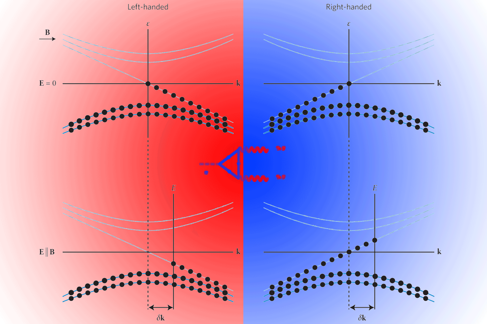
The ABJ anomaly: The electrons transfer from the neighborhood of the $LH$ degeneracy point to the $RH$ one in energy-momentum space.
2 (1+1)-dimensional and (3+1)-dimensional versions
In a theory of two Weyl spinors $\psi_\pm$ \[ \mathcal{L}=i\overline{\psi}/\kern-0.57em\partial\psi=i\psi^\dagger_+\sigma^\mu_+\partial_\mu\psi_++i\psi^\dagger_-\sigma^\mu_-\partial_\mu\psi_-\qquad\text{with}\quad\psi=\pmatrix{\psi_+\\ \psi_-} \]
Note: For convinience, we somethimes write $\psi_{R,L}$ as $\psi_{\pm}$.
The Lagrangian is easy to verify since we can get EOM from the Euler-Lagrange equations \[ \partial_\mu\left[\frac{\partial\mathcal{L}}{\partial(\partial_\mu\psi)}\right]-\frac{\mathcal{L}}{\partial\psi}=0 \] We get \[ \begin{align} \partial_\mu\left[\frac{\partial\mathcal{L}}{\partial(\partial_\mu\psi)}\right]-\frac{\mathcal{L}}{\partial\psi}&=\partial_\mu\left[\frac{\partial\mathcal{L}}{\partial(\partial_\mu\psi)}\right]\
&=\partial_\mu\left[\frac{\partial\left(i\psi^\dagger\gamma^0\gamma^\nu\partial_\nu\psi\right)}{\partial(\partial_\mu\psi)}\right]\
&=\partial_\mu\left[i\psi^\dagger\gamma^0\gamma^\nu\delta_{\mu\nu}\right]\
&=i\psi^\dagger\partial_\mu\gamma^0\gamma^\mu\
\end{align} \] where $\partial_\mu$ acts on the left, take the conjugation we get \[ -i(\gamma^\mu)^\dagger(\gamma^0)^\dagger\partial_\mu\psi=-i\gamma^0\gamma^\mu\partial_\mu\psi=0 \] where we use the relation $(\gamma^0)^\dagger=\gamma^0$, $(\gamma^\mu)^\dagger\gamma^0=\gamma^0\gamma^\mu$.
Multiplying this equation on the left by $-\gamma^0$ we get the EOM \[ i\gamma^\mu\partial_\mu\psi=0 \] where we use the relation $\gamma^0\gamma^0=1$.
The Lagrangian $\mathcal{L}$ is invariant under two types of global $U(1)$ transformations. In the first one both chiralities transform with the same phase, this is a vector transformation: \[ U(1)_V:\psi_\pm\to e^{i\alpha}\psi_\pm \] whereas in the second one, the axial $U(1)$, the signs of the phases are different for the two chiralities \[ U(1)_A:\psi_\pm\to e^{\pm i\alpha}\psi_\pm \]
Using Noether’s theorem, there are two conserved currents, a vector current \[ J^\mu_V=\overline{\psi}\gamma^\mu\psi\Longrightarrow\partial_\mu J^\mu_V=0 \] and an axial vector current \[ J^\mu_A=\overline{\psi}\gamma^\mu\gamma_5\psi\Longrightarrow\partial_\mu J^\mu_A=0 \]
Supplement: Noether’s theorem
Noether’s (first) theorem states that every differentiable symmetry of the action of a physical system has a corresponding conservation law.
Reference: Noether’s theorem - Wikipedia
The theory described by the Lagrangian $\mathcal{L}$ can be coupled to the electromagnetic field. The resulting classical theory is still invariant under the vector and axial $U(1)$ symmetries. Surprisingly, upon quantization it turns out that the conservation of the axial vector current is spoiled by quantum effects \[ \partial_\mu J^\mu_A\sim\hbar\mathbf{E}\cdot\mathbf{B}. \]
2.1 (1+1)-dimensions
To understand more clearly how this result comes about, we study first a simple model in two dimensions$(x^0,x^1)\equiv(t,x)$ that captures the relevant physics involved in the fourdimensional case. In two dimensions the dimension of the representation of the $\gamma$-matrices is 2. We have the following representation \[ \gamma^0\equiv\sigma_1=\pmatrix{0& 1\\ 1 & 0},\quad \gamma^1\equiv i\sigma_2=\pmatrix{0& 1\\ -1& 0}. \]
This is a chiral representation since the matrix $\gamma_5$ is diagonal \[ \gamma_5\equiv-\gamma^0\gamma^1=\pmatrix{1& 0\\ 0& -1}. \]
Writing a two-component Dirac spinor $\psi$ as \[ \psi=\pmatrix{\psi_R\\ \psi_L} \] and the projectors $P_\pm=\frac{1}{2}(1\pm\gamma_5)$ , and the components $\psi_{R,L}$ are respectively right- and left-handed Weyl spinors in two dimensions. Once we have a representation of the $\gamma$-matrices we can write the Weyl equation \[ i\gamma^\mu\partial_\mu\psi=0. \]
Expressed in terms of the components $\psi_{R,L}$ of the Dirac spinor, we have \[ (\partial_t-\partial_x)\psi_R=0,\quad (\partial_t+\partial_x)\psi_L=0. \]
In[9]:= pde=D[y[x,t],t]- D[y[x,t],x]==0
Out[9]= (y^(0,1))[x,t]-(y^(1,0))[x,t]==0
In[10]:= soln=DSolve[pde,y[x,t],{x,t}]
Out[10]= y[x,t]->C[1][t+x]
In[12]:= pde=D[y[x,t],t]+ D[y[x,t],x]==0
Out[12]= (y^(0,1))[x,t]+(y^(1,0))[x,t]==0
In[13]:= soln=DSolve[pde,y[x,t],{x,t}]
Out[13]= y[x,t]->C[1][t-x]
The general solution of these equations can be immediately written as \[ \psi_R=\psi_R(t+x),\quad \psi_L=\psi_L(t-x). \]
Hence $\psi_\pm$ are two wave packets moving along the spatial dimension respectively to the left $(\psi_R)$ and to the right ($\psi_L$). Notice that according to our convention the left-moving $\psi_R$ is a right-handed spinor (positive helicity) whereas the right-moving $\psi_L$ is a left-handed spinor (negative helicity).
Since we have $\gamma^\mu\partial_\mu\psi=(\gamma^0\partial_t+\gamma^1\partial_x)\psi=0$, by applying this twice we get the classical wave equation: \[ (\partial^2_t-\partial^2_x)\psi=0, \] where we use the relations $\gamma^0\gamma^0=I$, $\gamma^1\gamma^1=-I$ and $\{\gamma^0, \gamma^1\}=0$. Thus, both the left and right going components $\psi_L$ and $\psi_R$ obey the classical wave equation.
If we insist in interpreting the equation above as the wave equation for two-dimensional Weyl spinors, we expect the time dependence to be like $\exp(-iEt)$ where $E$ is the eigenvalue of the Hamiltonian and the spatial dependence to be that of a plane wave, that is, $\exp(ip\cdot x)$ for momentum $p$. In other words, our solution should be in this form \[ Ne^{-i(Et-p\cdot x)}=Ne^{-ip^\mu x_\mu}. \]
We find the following properly normalized wave functions for free particles with well defined energy-momentum $p^\mu=(E,p)$ \[ \phi_\pm(t\pm x)=\frac{1}{\sqrt{L}}e^{-iE(t\pm x)}, \qquad\text{with}\quad p=\mp E \]
As it is always the case with a relativistic wave equation, we have found both positive and negative energy solutions. For $\phi^{(E)}_{+}$, since $E=−p$, we see that the solutions with positive energy are those with negative momentum $p<0$, whereas the negative energy solutions are plane waves with $p>0$. For the left-handed spinor $\phi_{-}$ the situation is reversed. Besides, since the spatial direction is compact with length $L$ the momentum $p$ is quantized according to \[ p=\frac{2\pi n}{L},\quad n\in\mathbb{Z}. \]
The spectrum of the theory is represented in fig 1.
 |
|---|
| Fig 1: Spectrum of the massless two-dimensional Dirac field. We denote by $\phi_\pm$ the states with dispersion relation $E = \mp p$ |
Knowing the spectrum of the theory the next step is to obtain the vacuum. As with the Dirac equation in four dimensions, we identify the ground state of the theory with the one where all states with $E\leqslant0$ are filled(see the figure below).
 |
|---|
| Fig 2: The two branches in the vacuum of the theory. The solid points represent the filled negative energy states |
Exciting a particle in the Dirac sea produces a positive energy fermion plus a hole that is interpreted as an antiparticle. This gives us the key on how to quantize the theory. In the expansion of the operator $\psi_\pm$ we associate positive energy states with annihilation operators, whereas the states with negative energy are associated with creation operators for the corresponding antiparticle. \[ \psi_\pm(x)=\sum_{E>0}\left[a_\pm(E)\phi_\pm^{(E)}(x)+b_\pm^\dagger(E)\phi_\pm^{(E)}(x)^*\right]. \]
The operator $a_\pm(E)$ annihilates a particle with positive energy $E$ and momentum $\mp E$, and $b_\pm^\dagger(E)$ creates out of the vacuum an antiparticle with positive energy $E$ and spatial momentum $\mp E$. In the Dirac sea picture the operator $b_\pm^\dagger(E)$ is originally an annihilation operator for a state of the sea with negative energy $−E$. As in four dimensions, the problem of the negative energy states is solved by interpreting annihilation operators for negative energy states as creation operators for the corresponding antiparticle with positive energy (and vice versa). The operators appearing in the expansion of $\psi_\pm$ satisfy the usual fermionic algebra \[ \{a_\lambda(E),a_{\lambda’}^\dagger(E’)\}=\{b_\lambda(E),b_{\lambda’}^\dagger(E’)\}=\delta_{E,E’}\delta_{\lambda,\lambda’}, \] where we have introduced the label $\lambda, \lambda’=\pm$. In addition, $a_\lambda(E)$, $a_\lambda^\dagger(E)$ anticommute with $b_{\lambda’}(E)$, $b_{\lambda’}^\dagger(E)$.
Let’s take a very ad hoc approach to comping up the framework for a theory of many-particle systems using states in Fock space. We begin with two special cases.
- vacuum: $|0,0,\ldots,0,\ldots\rangle\equiv|\mathbf{0}\rangle$
- single-particle state: $|0,0,\ldots,n_i=1,\ldots\rangle\equiv|k_i\rangle$
Now we need to learn how to build multiparticle states while keeping the permutation symmetry. We define a “field operator” $a^{\dagger}_i$ that increases by one the number of particles in the state with eigenvalue $k_i$—that is \[ a^{\dagger}_i|n_1,n_2,\ldots,n_i,\ldots\rangle\propto|n_1,n_2,\ldots,n_i+1,\ldots\rangle \] We postulate that the action of the particle creation operator $a^{\dagger}_i$ on the vacuum is to create a proper normalized single-particle state, namely \[ a^{\dagger}_i|\mathbf{0}\rangle=|k_i\rangle, \] This lead us to write \[ \begin{align} 1=\langle k_i|k_i\rangle&=[\langle\mathbf{0}|a_i][a^{\dagger}_i|\mathbf{0}\rangle]\
&=\langle\mathbf{0}|\left[a_ia^{\dagger}_i|\mathbf{0}\rangle\right]=\langle\mathbf{0}|a_i|k_i\rangle \end{align} \] which implies that $a_i|k_i\rangle=|\mathbf{0}\rangle$ so that $a_i$ act as a particle annihilation operator \[ a_i|n_1,n_2,\ldots,n_i,\ldots\rangle\propto|n_1,n_2,\ldots,n_i-1,\ldots\rangle \] and $a_i|\mathbf{0}\rangle=0$ as well as $a_i|k_j\rangle=\delta_{ij}|\mathbf{0}\rangle$.
For a two-particle state, that act of permuting two particle(bosons, fermions) can be in this way \[ a^{\dagger}_i a^{\dagger}_j|\mathbf{0}\rangle=\pm a^{\dagger}_j a^{\dagger}_i|\mathbf{0}\rangle \] We are led to \[ \begin{align} a^{\dagger}_i a^{\dagger}_j-a^{\dagger}_j a^{\dagger}_i=[a^{\dagger}_i, a^{\dagger}_j]=0&\qquad\text{Bosons}\
a^{\dagger}_i a^{\dagger}_j+a^{\dagger}_j a^{\dagger}_i=\{a^{\dagger}_i, a^{\dagger}_j\}=0&\qquad\text{Fermions} \end{align} \] Simply taking the adjiont of these equations tells us that \[ \begin{align} [a_i, a_j]=0&\qquad\text{Bosons}\
\{a_i, a_j\}=0&\qquad\text{Fermions} \end{align} \] To get the commutations rules for $a_i$ and $a^{\dagger}_j$ we would like to define a “number operator” $N_i=a^{\dagger}_i a_i$ that would count the number of particles in the state $|k_i\rangle$. This would be possible if we have \[ \begin{align} [a_i, a^{\dagger}_j]=\delta_{ij}&\qquad\text{Bosons}\
\{a_i, a^{\dagger}_j\}=\delta_{ij}&\qquad\text{Fermions} \end{align} \]
The Lagrangian of the theory \[ \mathcal{L}=i\psi^\dagger_+(\partial_0+\partial_x)\psi_++i\psi^\dagger_-(\partial_0-\partial_x)\psi_- \] is invariant under both the $U(1)_V$ transformations and $U(1)_A$. The corresponding Noether currents are \[ J^\mu_V=\pmatrix{\psi^\dagger_+\psi_++\psi^\dagger_-\psi_-\\ -\psi^\dagger_+\psi_++\psi^\dagger_-\psi_-},\quad J^\mu_A=\pmatrix{\psi^\dagger_+\psi_+-\psi^\dagger_-\psi_-\\ -\psi^\dagger_+\psi_+-\psi^\dagger_-\psi_-} \]
The associated conserved charges are given by \[ Q_V\equiv\int_0^LdxJ_V^0=\int_0^Ldx\left(\psi^\dagger_+\psi_++\psi^\dagger_-\psi_-\right), \] for the vector current, and \[ Q_A\equiv\int_0^LdxJ_A^0=\int_0^Ldx\left(\psi^\dagger_+\psi_+-\psi^\dagger_-\psi_-\right), \]
for the vector axial one. Using the orthonormality relations for the modes $\phi^{(E)}_\pm(x)$ \[ \int_0^Ldx\phi^{(E)}_\pm(x)^*\phi^{(E’)}_\pm(x)=\delta_{E,E’}, \] the conserved charges can be explicitly computed as \[ \begin{align} Q_V&=\sum_{E>0}\left[a^\dagger_+(E)a_+(E)-b^\dagger_+(E)b_+(E)+a^\dagger_-(E)a_-(E)-b^\dagger_-(E)b_-(E)\right],\
Q_A&=\sum_{E>0}\left[a^\dagger_+(E)a_+(E)-b^\dagger_+(E)b_+(E)-a^\dagger_-(E)a_-(E)+b^\dagger_-(E)b_-(E)\right]. \end{align} \]
From these expressions we see how $Q_V$ counts the net fermion number, i.e. the number of particles minus antiparticles, independently of their helicity. The axial charge $Q_A$, on the other hand, counts the net number of positive minus negative helicity states. In the case of the vector current we have subtracted a formally divergent vacuum contribution to the charge (the “charge of the Dirac sea”).
In the free theory there is of course no problem with the conservation of either $Q_V$ or $Q_A$, since the occupation numbers do not change. What we want to study is the effect of coupling the theory to the uniform electric field $\dot{A^1}=E$ in the temporal gauge. We have already know that \[ \mathbf{E}=-(\partial_t\mathbf{A}+\nabla A^0),\quad\mathbf{B}=\nabla\times\mathbf{A} \]
We work in the gauge $A^0=0$. The one component RH Weyl equation reads \[ i\dot{\psi}_R(x)=(-i\partial_x-A^1)\psi_R(x). \]
Instead of solving the problem exactly we are going to use the following trick: we simulate the electric field by adiabatically varying in a long time $\tau_0$ the vector potential $A^1$ from zero value to $E\tau_0$. we know that the effect of the electromagnetic coupling in the theory is a shift in the momentum according to \[ p\to p-eA^1, \] where $e$ is the charge of the fermions. Since we assumed that the vector potential varies adiabatically, we can take it to be approximately constant at each time.
We have to understand the effect on the vacuum depicted in Fig 2 of switching on the vector potential. Increasing adiabatically $A^1$ results in decreasing the momentum of the state. What happens to the energy depends on whether we consider states with dispersion relation $E = −p$ (the branch $\phi_+$) or $E = p$ (the branch $\phi_-$).
 |
|---|
| Fig 3: Effect of the electric field on the vacuum. Some of the occupied negative energy states in the brach $\phi_+$ acquires positive energy, while the same number of empty positive energy states in the branch $\phi_-$ shift to negative energy and become holes in the Dirac sea |
The result is that the two branches move as shown in Fig 3. Thus, some of the negative energy states of the $\phi_+$ branch acquire positive energy while the same number of the empty positive energy states of the other branch $\phi_-$ become empty negative energy states. Physically, this means that the external electric field $E$ creates a number of particle-antiparticle pairs out of the vacuum.
We have to count the number of such pairs created by the electric field after a time $\tau_0$. This is given by \[ N=eE\tau_0\cdot\frac{L}{2\pi}=\frac{L}{2\pi}eE\tau_0 \] where $L/2\pi$ is DOS. The value of the charges at the time $\tau_0$ are \[ \begin{align} Q_V(\tau_0)&=(N-0)+(0-N)=0,\
Q_A(\tau_0)&=(N-0)-(0-N)=2N. \end{align} \]
We conclude that the coupling to the electric field produces a violation in the conservation of the axial charge per unit time given by \[ \dot{Q}_A=\frac{2N}{\tau_0}=\frac{e}{\pi}EL. \]
This result translates into a nonconservation of the axial vector current \[ \partial_\mu J^\mu_A=\frac{1}{L}\dot{Q}_A=\frac{e}{\pi}E. \]
In addition, the fact that $\Delta Q_V=0$ guarantees that the vector current remains conserved also quantum mechanically, $\partial_\mu J^\mu_V=0$.
2.2 (3+1)-dimensions
In 3+1 dimensions we first calculate the energy levels of the RH Weyl fermion in the presence of the applied uniform magnetic field $\mathbf{B}=H\hat{e}_3=\nabla\times\mathbf{A}$ along the third direction given by \[ A^\mu=\pmatrix{0\\ 0\\ Hx^1\\ 0} \]
2.2.1 Dirac oscillator method
The solution to the equation for a two-component RH field $\psi_R$ of the form \[ \left[i\partial/\partial t-(\mathbf{p}-e\mathbf{A})\cdot\boldsymbol{\sigma}\right]\psi_R(\mathbf{x})=0 \] with the Hamiltonian \[ \mathcal{H}=(\mathbf{p}-e\mathbf{A})\cdot\boldsymbol{\sigma} \] is expressed in terms of a solution of the auxiliary equation \[ \left[i\partial/\partial t-(\mathbf{p}-e\mathbf{A})\cdot\boldsymbol{\sigma}\right]\left[i\partial/\partial t+(\mathbf{p}-e\mathbf{A})\cdot\boldsymbol{\sigma}\right]\Phi=0\tag{5} \] as \[ \psi_R=\left[i\partial/\partial t+(\mathbf{p}-e\mathbf{A})\cdot\boldsymbol{\sigma}\right]\Phi. \]
Let’s calculate eq (5) explicitly. \[ (5)\Longrightarrow\left\{-\partial_t^2-[(\mathbf{p}-e\mathbf{A})\cdot\boldsymbol{\sigma}][(\mathbf{p}-e\mathbf{A})\cdot\boldsymbol{\sigma}]\right\}\Phi=0 \]
Using the relation $\omega\longleftrightarrow i\partial_t$ we get \[ \left\{[(\mathbf{p}-e\mathbf{A})\cdot\boldsymbol{\sigma}][(\mathbf{p}-e\mathbf{A})\cdot\boldsymbol{\sigma}]\right\}\Phi=\omega^2\Phi \]
Then we expand the left side of the equation above \[ \begin{align} \mathrm{I}=&\left\{[(\mathbf{p}-e\mathbf{A})\cdot\boldsymbol{\sigma}][(\mathbf{p}-e\mathbf{A})\cdot\boldsymbol{\sigma}]\right\}\
=&(p^i-eA^i)\sigma_i(p^j-eA^j)\sigma_j\
=&\sigma_i\sigma_j(p^i-eA^i)(p^j-eA^j)\
=&\left(\frac{1}{2}\{\sigma_i, \sigma_j\}+\frac{1}{2}[\sigma_i, \sigma_j]\right)(p^i-eA^i)(p^j-eA^j)\
=&(\delta_{ij}+i\epsilon_{ijk}\sigma_k)(p^i-eA^i)(p^j-eA^j)\
=&\underbrace{(p^i-eA^i)(p^i-eA^i)}_{\mathrm{I_1}}+\underbrace{i\epsilon_{ijk}\sigma_k(p^i-eA^i)(p^j-eA^j)}_{\mathrm{I_2}} \end{align} \] where we have use the relations $\{\sigma_i, \sigma_j\}=2\delta_{ij}$ and $[\sigma_i, \sigma_j]=2i\epsilon_{ijk}\sigma_k$. Let’s go on \[ \mathrm{I_1}=(p^1)^2+(p^2-eHx^1)^2+(p^3)^2 \] and \[ \begin{align} \mathrm{I_2}=&\quad i\sigma_1\left[(p^2-eHx^1)p^3-p^3(p^2-eHx^1)\right]\
&+i\sigma_2\left[p^3p^1-p^1p^3\right]\
&+i\sigma_3\left[p^1(p^2-eHx^1)-(p^2-eHx^1)p^1\right]\
=&\quad i\sigma_1\left([p^2, p^3]-eH[x^1, p^3]\right)\
&+i\sigma_2\left[p^3, p^1\right]\
&+i\sigma_3\left([p^1, p^2]+eH[x^1, p^1]\right)\
=&i\sigma_3eHi\hbar\
=&-eH\sigma_3 \end{align} \] where we have use the relations $[x_i,p_j]=i\hbar\delta_{ij}$ and $[p_i, p_j]=0$.
Combing $\mathrm{I_1}$ and $\mathrm{I_2}$ we get \[ \left[(p^1)^2+(p^2-eHx^1)^2+(p^3)^2-eH\sigma_3\right]\Phi=\omega^2\Phi \]
Using tensor analysis, we can also derive the result \[ \begin{align} &(\tilde{\mathbf{p}}\cdot\boldsymbol{\sigma})(\tilde{\mathbf{p}}\cdot\boldsymbol{\sigma})\Phi\
=&\left[\tilde{\mathbf{p}}^2+i\boldsymbol{\sigma}\cdot(\tilde{\mathbf{p}}\times\tilde{\mathbf{p}})\right]\Phi\
=&(\tilde{\mathbf{p}}^2-\boldsymbol{\sigma}\cdot e\mathbf{B})\Phi \end{align} \] where we define $\tilde{\mathbf{p}}\equiv\mathbf{p}-e\mathbf{A}$ for simplicity, and use the relations \[ (\mathbf{a}\cdot\boldsymbol{\sigma})(\mathbf{b}\cdot\boldsymbol{\sigma})=\mathbf{a}\cdot\mathbf{b}+i\boldsymbol{\sigma}\cdot(\mathbf{a}\times\mathbf{b}) \] as well as \[ \begin{align} \tilde{\mathbf{p}}\times\tilde{\mathbf{p}}\Phi&=(i\nabla+e\mathbf{A})\times(i\nabla\Phi+e\mathbf{A}\Phi)\
&=ie[\nabla\times(\mathbf{A}\Phi)+\mathbf{A}\times\nabla\Phi]\
&=ie(\nabla\times\mathbf{A})\Phi\
&=ie\mathbf{B}\Phi. \end{align} \]
The eigenfunction above satisfies an equation of the harmonic oscillator type. The operator $p^2$ and $p^3$ commute with the left side since they are absent by the choice of gauge. Thus they can be replaced by their eigenvalues $p^2$ and $p^3$ with eigenfunction $e^{-ip_2x^2}$ and $e^{-ip_3x^3}$.
Let’s construct the annihilation operator \[ a_{p^2}=\sqrt{\frac{eH}{2}}\left([x^1-\frac{p^2}{eH}]+i\frac{p^1}{eH}\right) \] and the creation operator \[ a_{p^2}^\dagger=\sqrt{\frac{eH}{2}}\left([x^1-\frac{p^2}{eH}]-i\frac{p^1}{eH}\right). \]
It is easy to check \[ \begin{align} [a_{p^2},a_{p^2}^\dagger]&=\frac{eH}{2}\left([x^1,-i\frac{p^1}{eH}]+[i\frac{p^1}{eH},x^1]\right)\
&=\frac{eH}{2}\left(-\frac{i}{eH}[x^1,p^1]-\frac{i}{eH}[x^1,p^1]\right)\
&=\frac{eH}{2}\left(-\frac{i}{eH}i-\frac{i}{eH}i\right)\
&=1 \end{align} \] and \[ \begin{align} a_{p^2}^\dagger a_{p^2}&=\frac{eH}{2}\left((\frac{p^1}{eH})^2+(x^1-\frac{p^2}{eH})^2+[x^1,i\frac{p^1}{eH}]\right)\
&=\frac{eH}{2}\left((\frac{p^1}{eH})^2+(\frac{p^2}{eH}-x^1)^2-\frac{1}{eH}\right)\
&=\frac{eH}{2}\left((\frac{p^1}{eH})^2+(\frac{p^2}{eH}-x^1)^2\right)-\frac{1}{2} \end{align} \] which we define as the number operator $N$, we denote an eigenket of $N$ by its eigenvalue $n$, so \[ N|n\rangle=n|n\rangle \]
Thus, we get \[ \begin{align} \mathrm{I}\Phi&=\left[(p^1)^2+(p^2-eHx^1)^2+(p^3)^2-eH\sigma_3\right]\Phi\
&=\left[2eH\frac{eH}{2}\left((\frac{p^1}{eH})^2+(\frac{p^2}{eH}-x^1)^2\right)+(p^3)^2-eH\sigma_3\right]\Phi\
&=\left[2eH(a_{p^2}^\dagger a_{p^2}+\frac{1}{2})+(p^3)^2-eH\sigma_3\right]\Phi\
&=\left[2eH(N+\frac{1}{2})+(p^3)^2-eH\sigma_3\right]\Phi \end{align} \]
Because $\mathrm{I}$ is just a linear function of $N$, $N$ can be diagonalized simultaneously with $\mathrm{I}$. We have \[ \begin{align} \mathrm{I}|n\rangle&=\left[2eH(N+\frac{1}{2})+(p^3)^2-eH\sigma_3\right]|n\rangle\
&=\left[2eH(n+\frac{1}{2})+(p^3)^2-eH\sigma_3\right]|n\rangle\
&=\omega^2|n\rangle \end{align} \]
To appreciate the physical significance of $a_{p^2}$, $a_{p^2}^\dagger$ and $N$, let’s first note that \[ [N,a]=[a^\dagger a,a]=a^\dagger[a,a]+[a^\dagger,a]a=-a \] where we use the relation $[AB,C]=A[B,C]+[A,C]B$.
Likewise, we can derive \[ [N,a^\dagger]=a^\dagger \]
As a result, we have \[ Na^\dagger|n\rangle=([N,a^\dagger]+a^\dagger N)|n\rangle=(n+1)a^\dagger|n\rangle \] and \[ Na|n\rangle=([N,a]+aN)|n\rangle=(n-1)a|n\rangle. \]
These relations imply that $a^\dagger|n\rangle$(or $a|n\rangle$) is also an eigenket of $N$ with eigenvalue increases(decreases) by one. Compared with the eigenket of $N$ we can see that $a|n\rangle$ and $|n-1\rangle$ are the same up to a mutiplicative constant. We write \[ a|n\rangle=c|n-1\rangle \]
Note that \[ \langle n|a^\dagger a|n\rangle=|c|^2 \] since $N=a^\dagger a$, we get \[ n=|c|^2 \]
Taking $c$ to be real and positive by convention, we obtain \[ a|n\rangle=\sqrt{n}|n-1\rangle \]
Similarly, it is easy to show that \[ a^\dagger|n\rangle=\sqrt{n+1}|n+1\rangle \]
Suppose that we keep on applying the annihilation operator $a$ on the eigenket, we can obtain smaller and smaller $n$ until the sequence terminates. That means $n$ must be a nonnegative integer since we have \[ n=\langle n|N|n\rangle=(\langle n|a^\dagger)\cdot (a|n\rangle)\geqslant0. \]
The sequence terminates with $n=0$, which means $a|0\rangle=0$. We can now successively apply the creation operator $a^\dagger$ to the ground state $|0\rangle$ to obtain \[ |n\rangle=\left[\frac{(a^\dagger)^n}{\sqrt{n!}}\right]|0\rangle. \]
Let us find the eigenfunctions with the ground state \[ a|0\rangle=0 \] which, in $x^1$-representation, reads \[ \langle x’^1|a|0\rangle=\sqrt{\frac{eH}{2}}\langle x’^1|\left([x^1-\frac{p^2}{eH}]+i\frac{p^1}{eH}\right)|0\rangle=0 \] using the relation $\langle x’|p|0\rangle=-i\frac{\partial}{\partial x’}\langle x’|0\rangle$ we get \[ \left([x’^1-\frac{p^2}{eH}]+\frac{1}{eH}\frac{d}{d x’^1}\right)\langle x’^1|0\rangle=0. \]
Let $\xi\equiv x’^1-\frac{p^2}{eH}$ and $u(\xi)=\langle x’^1|0\rangle$, we get \[ \frac{d u}{d\xi}=-eH\xi u \]
This differential equation is easy to solve \[ \int\frac{d u}{u}=-eH\int\xi d\xi\Longrightarrow \ln u=-\frac{eH}{2}\xi^2+\text{constant} \] so \[ u(\xi)=Ae^{-\frac{eH}{2}\xi^2}. \]
We might as well normalize it right away \[ 1=|A|^2\int e^{-eH\xi^2}d\xi=|A|^2\sqrt{\frac{\pi}{eH}} \] so $|A|^2=\sqrt{eH/\pi}$, and hence \[ \langle x^1|0\rangle=\left(\frac{eH}{\pi}\right)^{1/4}e^{-\frac{eH}{2}(x^1-\frac{p^2}{eH})^2}. \]
In general, we obtain \[ \langle x^1|n\rangle=\langle x^1|\left[\frac{(a^\dagger)^n}{\sqrt{n!}}\right]|0\rangle=\frac{1}{\sqrt{n!}}\left(\sqrt{\frac{eH}{2}}\right)^n\left([x^1-\frac{p^2}{eH}]-\frac{1}{eH}\frac{d}{d x^1}\right)^n\langle x’^1|0\rangle \]
Using the physicists’ Hermite polynomials $H_n$ \[ H_{n}(z)=(-1)^{n}~e^{z^{2}}{\frac {d^{n}}{dz^{n}}}\left(e^{-z^{2}}\right) \] we get \[ \langle x^1|n\rangle=\phi_{n}(x)={\frac {1}{\sqrt {2^{n}\,n!}}}\cdot \left({\frac {eH}{\pi}}\right)^{1/4}\cdot e^{-\frac{eH}{2}(x^1-\frac{p^2}{eH})^2}\cdot H_{n}\left({\sqrt {eH}}x^1-\frac{p^2}{\sqrt{eH}}\right) \] where $n=0,1,2,\ldots$. The first eleven physicists’ Hermite polynomials are: \[ \begin{aligned}H_{0}(x)&=1\
H_{1}(x)&=2x\
H_{2}(x)&=4x^{2}-2\
H_{3}(x)&=8x^{3}-12x\
H_{4}(x)&=16x^{4}-48x^{2}+12\
H_{5}(x)&=32x^{5}-160x^{3}+120x\
H_{6}(x)&=64x^{6}-480x^{4}+720x^{2}-120\
H_{7}(x)&=128x^{7}-1344x^{5}+3360x^{3}-1680x\
H_{8}(x)&=256x^{8}-3584x^{6}+13440x^{4}-13440x^{2}+1680\
H_{9}(x)&=512x^{9}-9216x^{7}+48384x^{5}-80640x^{3}+30240x\
H_{10}(x)&=1024x^{10}-23040x^{8}+161280x^{6}-403200x^{4}+302400x^{2}-30240. \end{aligned} \]
Reference: Wikipedia: Hermite polynomials
It is time to conclude the discussions above. Let us write the equation again \[ \mathrm{I}\Phi=\left[2eH(N+\frac{1}{2})+(p^3)^2-eH\sigma_3\right]\Phi. \]
$\Phi$ can be write as $\phi_n\phi_{p^2}\phi_{p^3}$, where $\phi_n$, $\phi_{p^2}$ and $\phi_{p^3}$ are eigenfuntions of $N$, $p^2$, $p^3$ which commute with each other. Let us write them explicitly \[ \begin{align} N\phi_N&=n\phi_{n}(x)\
p^2\phi_{p^2}&=p^2e^{ip^2x^2}\
p^3\phi_{p^3}&=p^3e^{ip^3x^3}\
\end{align} \]
Finally, we get the solution of $\mathrm{I}\Phi=\omega^2\Phi$: \[ \omega^2(n, \sigma_3, p^3)=2eH(n+\frac{1}{2})+(p^3)^2-eH\chi_{\sigma_3} \] and \[ \Phi_{n\sigma_3}=\phi_n\phi_{p^2}\phi_{p^3}\chi(\sigma_3) \] where $\chi(\sigma_3)$ denotes the eigenfunctions of the Pauli spin $\sigma_3$ which can be taken as $\chi(1)=\pmatrix{1\\ 0}$ and $\chi(-1)=\pmatrix{0\\ 1}$ and $\chi_{\sigma_3}$ is the corresponding eigenvalue $\pm1$.
Now, we need to find the interpretation of the solutions above. For each $\Phi_{n\sigma_3}$, the eigenvalues $\omega(n, \sigma_3, p^3)$ are included. On the other hand, the negative eigenvalues $-\omega(n, \sigma_3, p^3)$ are also included. This remainds us of the situations when interpreting Klein-Gordon equation where we defined a two component object $\Upsilon=\pmatrix{\phi\\ \chi}$ and interpreted $\phi$ as the wave function of a positive particle while $\chi$ of negative particle. But here, where the addtional degree of freedom comes from? We will leave this problem for the discussion before long.
It is easy to get $\psi_R$ using the relation \[ \begin{align} \psi_R&=\left[i\partial/\partial t+(\mathbf{p}-e\mathbf{A})\cdot\boldsymbol{\sigma}\right]\Phi_{n\sigma_3}\
&=\pmatrix{i\partial_t+p^3& p^1-i(p^2-eHx^1)\\ p^1+i(p^2-eHx^1)& i\partial_t-p^3}\Phi_{n\sigma_3}\
&=\pmatrix{i\partial_t+p^3& i\sqrt{2eH}a_{p^2}^\dagger\\ -i\sqrt{2eH}a_{p^2}& i\partial_t-p^3}\Phi_{n\sigma_3} \end{align} \]
Then we can see that \[ \psi_{R_{n,\chi_{\sigma_3}=+1}}=\left\{ \begin{align} &\pmatrix{(\omega+p^3)\phi_n\phi_{p^2}\phi_{p^3}\\ -i\sqrt{2eH}\sqrt{n}\phi_{n-1}\phi_{p^2}\phi_{p^3}}&\quad\text{for }n\geqslant1\
&\pmatrix{(\omega+p^3)\phi_0\phi_{p^2}\phi_{p^3}\\ 0}&\quad\text{for }n=0 \end{align}\right. \] and \[ \psi_{R_{n,\chi_{\sigma_3}=-1}}=\pmatrix{i\sqrt{2eH}\sqrt{n+1}\phi_{n+1}\phi_{p^2}\phi_{p^3}\\ (\omega-p^3)\phi_n\phi_{p^2}\phi_{p^3}}\quad\text{for }n\geqslant0 \] where we use the relations $a\phi_n=\sqrt{n}\phi_{n-1}$, $a^\dagger\phi_n=\sqrt{n+1}\phi_{n+1}$ and $a\phi_0=0$. Take a closer look we can see for $n\geqslant0$ \[ \psi_{R_{n+1,\chi_{\sigma_3}=+1}}=\psi_{R_{n,\chi_{\sigma_3}=-1}} \] with the same energy eigenvalue \[ \omega=\pm\sqrt{2eH(n+1)+(p^3)^2}. \]
This means $\psi_{R_{n+1,\chi_{\sigma_3}=+1}}$ and $\psi_{R_{n,\chi_{\sigma_3}=-1}}$ are the same state. However, the poor $\psi_{R_{0,\chi_{\sigma_3}=+1}}$ doesn’t have a parterner($\chi_{\sigma_3}=-1$). Let us give special attention to this single one before we take it for granted that its dispersion law is $\pm p^3$. Our intuition is telling us that something goes different here. We’d better use the original equation to check the energy eigenvalue. \[ \left[i\partial/\partial t-(\mathbf{p}-e\mathbf{A})\cdot\boldsymbol{\sigma}\right]\psi_R=0 \]
Write this equation in ladder operator form \[ \begin{align} &\left[i\partial/\partial t-(\mathbf{p}-e\mathbf{A})\cdot\boldsymbol{\sigma}\right]\psi_R\
=&\pmatrix{i\partial_t-p^3& -p^1+i(p^2-eHx^1)\\ -p^1-i(p^2-eHx^1)& i\partial_t+p^3}\psi_R\
=&\pmatrix{i\partial_t-p^3& -i\sqrt{2eH}a_{p^2}^\dagger\\ i\sqrt{2eH}a_{p^2}& i\partial_t+p^3}\psi_R\
=&\pmatrix{\omega-p^3& -i\sqrt{2eH}a_{p^2}^\dagger\\ i\sqrt{2eH}a_{p^2}& \omega+p^3}\psi_R\
=&\pmatrix{(\omega-p^3)\psi_{R_{\text{upper}}} -i\sqrt{2eH}a_{p^2}^\dagger\psi_{R_{\text{lower}}}\\ i\sqrt{2eH}a_{p^2}\psi_{R_{\text{upper}}} +(\omega+p^3)\psi_{R_{\text{lower}}}}\
=&0 \end{align} \] where $\psi_{R_{\text{upper}}}$ and $\psi_{R_{\text{lower}}}$ denotes the upper and lower component of $\psi_R$.
Now we can see it expicitly that only $\omega=+p^3$ is allowed for $\psi_{R_{0,\chi_{\sigma_3}=+1}}$(in other word, $\psi_{R_{0,\chi_{\sigma_3}=+1}}$=0 with $\omega=-p^3$). The reason is that $a_{p^2}^\dagger\psi_{R_{\text{lower}}}=0$ for $\psi_{R_{0,\chi_{\sigma_3}=+1}}$($a^\dagger$ cannot raise $0$ to $|0\rangle$ to counteract $\psi_{R_{\text{upper}}}$) and we need \[ (\omega-p^3)\psi_{R_{\text{upper}}} -i\sqrt{2eH}a_{p^2}^\dagger\psi_{R_{\text{lower}}}=(\omega-p^3)\psi_{R_{\text{upper}}}=0
\Longrightarrow\omega=+p^3 \]
But for $n\geqslant1$, the lower component of $\psi_{R_{n,\chi_{\sigma_3}=+1}}$ can always be lifted up, which results in $\omega=\pm\sqrt{2neH+(p^3)^2}$.
Next, we discuss the degeneracy of ground states. We would like to figure out how many states there are, assuming that the system has an overall finite size. Let us recall \[ \phi_{n}(x)={\frac {1}{\sqrt {2^{n}\,n!}}}\cdot \left({\frac {eH}{\pi}}\right)^{1/4}\cdot e^{-\frac{eH}{2}(x^1-\frac{p^2}{eH})^2}\cdot H_{n}\left({\sqrt {eH}}x^1-\frac{p^2}{\sqrt{eH}}\right). \]
Each Landau level is degenerate because of the second quantum number $p^2$, which can take the values \[ p^2=\frac{2\pi N_y}{L_y}. \] where $N_y$ is an integer. The allowed values of $N_y$ are further restricted by the condition that the center of force of the oscillator, $x^1_0\equiv\frac{p^2}{eH}$, must physically lie within the system, $0\leqslant x^1_0 < L_x$. This gives the following range for $N_y$, \[ 0\leqslant N_y<\frac{eHL_xL_y}{2\pi}. \]
Here $N$ denotes the number of states.
Thus we get the upper bound on $N$ \[ N=N_yN_z=\frac{eHL_xL_yL_z}{4\pi^2}. \] where we use the realtion $N_z=\frac{L_z}{2\pi}$.
Here $N_x$ is ommited because there is no degree of freedom left for it(Its effect is covered by $N_y$).
 |
|---|
| Fig 4: Dispersion law for the RH Weyl fermion in $3+1$ dimensions in the presence of a magnetic field in the $x^3$-direction. |
We close the discussion in this part with Fig 4 and continue our following discussion of another way to construct $\psi_R$.
2.2.2 Hamiltonian method
The Weyl equation is \[ \mathcal{H}\psi_R(\mathbf{x})=\omega\psi_R(\mathbf{x}) \] with the Hamiltonian \[ \mathcal{H}=(\mathbf{p}-e\mathbf{A})\cdot\boldsymbol{\sigma}. \]
This problem gets really simple based on our $a$ and $a^\dagger$ operators. We write the equation in this way \[ \pmatrix{p^3& i\sqrt{2eH}a_{p^2}^\dagger\\ -i\sqrt{2eH}a_{p^2}& -p^3}\psi_R=\omega\psi_R \]
We can get first the energy eigenvalue \[ \omega=\pm\sqrt{(p^3)^2+2neH},\quad n\geqslant1 \] from the eigenvalue equation \[ \omega^2=(p^3)^2+2eHa^\dagger a=(p^3)^2+2neH,\quad n\geqslant1 \] which requires that the two-component column vector function $\psi_R$ should be of this form \[ \psi_{R_n}=\pmatrix{\phi_n\phi_{p^2}\phi_{p^3}\\ \lambda\phi_{n-1}\phi_{p^2}\phi_{p^3}} \] because the Hamiltonian $\mathcal{H}$ is always raising the lower component of $\psi_R$ while lowering the upper one. Here we are merely interested in the ratio $\lambda$ of the upper to lower component and we can get it easily. From \[ \pmatrix{p^3& i\sqrt{2eH}a_{p^2}^\dagger\\ -i\sqrt{2eH}a_{p^2}& -p^3}\pmatrix{\phi_n\phi_{p^2}\phi_{p^3}\\ \lambda\phi_{n-1}\phi_{p^2}\phi_{p^3}}=\omega\pmatrix{\phi_n\phi_{p^2}\phi_{p^3}\\ \lambda\phi_{n-1}\phi_{p^2}\phi_{p^3}} \] we get $\lambda=\frac{\omega-p^3}{i\sqrt{2neH}}=\frac{-i\sqrt{2neH}}{\omega+p^3}$ for $n\geqslant1$.
This is consistent with $\psi_{R_{n,\chi_{\sigma_3}=+1}}$ and $\psi_{R_{n,\chi_{\sigma_3}=+1}}$ we abtain above.
When $n=0$, the energy eigenvalue is not \[ \omega=\pm p^3 \] but \[ \omega=+p^3. \] with the eigenfunction \[ \psi_{R_0}=\pmatrix{\phi_0\phi_{p^2}\phi_{p^3}\\ 0}. \]
The reason for our casting aside $\omega=-p^3$ is that $a\phi_0=0$ but $a^\dagger0\ne\phi_0$ which is not the situation for $n\geqslant1$ where $a\phi_n=\sqrt{n}\phi_{n-1}$ and $a^\dagger\phi_{n-1}=\sqrt{n}\phi_n$. Let us write it out explicitly \[ \pmatrix{p^3& i\sqrt{2eH}a_{p^2}^\dagger\\ -i\sqrt{2eH}a_{p^2}& -p^3}\pmatrix{\phi_0\phi_{p^2}\phi_{p^3}\\ 0}=p^3\pmatrix{\phi_0\phi_{p^2}\phi_{p^3}\\ 0}=\omega\pmatrix{\phi_0\phi_{p^2}\phi_{p^3}\\ 0}. \]
We are not surprised to find that $-p^3$ doesn’t even appear because the lower component is always zero, that is to say a degree of freedom(e.i. $\lambda$) is lost. This is consistent with the former discussion.
Here we give a simple discussion of a charged particle (electron) in a uniform magnetic field in QM. To simplify the setup, let us consider the electron to move only on $xy$ plane under a magnetic field pointing along the $z$ direction. If you use the canonical formalism, you need to specify the vector potential even in the classical mechanics. One common choice preserves the rotational invariance (the symmetric gauge) \[ \vec{A}=(A_x,A_y)=\frac{B}{2}. \] First important point is that two kinetic momenta do not commute \[ [\Pi_x,\Pi_y]=[p_x-\frac{e}{c}A_x,p_y-\frac{e}{c}A_y]=i\frac{e}{c}(\nabla_xA_y-\nabla_yA_x)=i\frac{e\hbar}{c}B_z \] We define the creation and annihilation operators by \[ \begin{align} a&=\sqrt{\frac{c}{2e\hbar B}}(\Pi_x+i\Pi_y)\
a^\dagger&=\sqrt{\frac{c}{2e\hbar B}}(\Pi_x-i\Pi_y) \end{align} \] They satisfy \[ [a,a^\dagger]=\frac{c}{2e\hbar B}[\Pi_x+i\Pi_y,\Pi_x-i\Pi_y]=1. \] The Hamiltonian is \[ \mathcal{H}=\hbar\omega(a^\dagger a+\frac{1}{2}) \] with the classical cyclotron frequency $\omega=\frac{eB}{mc}$. The spectrum is that of a harmonic oscillator \[ E=\hbar\omega(n+\frac{1}{2}) \] with $n$ a non-negative integer. The energy eigenstates are called Landau levels.
It is straightforward to include the electron spin into the Hamiltonian with the magnetic moment $\vec{\mu}=g\frac{e\vec{s}}{2mc}$, \[ \mathcal{H}=\hbar\omega(a^\dagger a+\frac{1}{2})-g\frac{e}{2mc}\vec{s}\cdot\vec{B}=\hbar\omega(a^\dagger a+\frac{1}{2}-\frac{g}{4}\sigma_z) \] where we used the relations $\omega=\frac{eB}{mc}$ and $s_z=\hbar\sigma_z/2$.
There is a remarkable point about the electron with $g = 2$. The ground states with $\sigma_z=+1$ has precisely zero energy, while the ground states with $\sigma_z=-1$ and the first Landau level with $\sigma_z=+1$ are degenerate(see fig 5).
Fig 5: The Landau levels with spin and $g = 2$. Each level is degenerate between the spin up and down states, while the ground state has precisely zero energy with only the spin up state.
This point can be understood by defining the operator \[ Q=\sqrt{\frac{1}{2m}}(\sigma_x\Pi_x+\sigma_y\Pi_y). \] The square of this operator is \[ \begin{align} Q^2&=\frac{1}{2m}\left(\Pi_x^2+\Pi_y^2+\sigma_x\sigma_y\Pi_x\Pi_y+\sigma_y\sigma_x\Pi_y\Pi_x\right)\
&=\frac{1}{2m}\left(\sigma_x^2\Pi_x^2+\sigma_y^2\Pi_y^2+i\sigma_z[\Pi_x,\Pi_y]\right)\
&=\frac{1}{2m}(\Pi_x^2+\Pi_y^2)-\frac{e\hbar B}{2mc}\sigma_z\
&=\mathcal{H} \end{align} \] precisely the Hamiltonian with $g=2$. One can further rewrite this operator as a matrix \[ \begin{align} Q&=\sqrt{\frac{1}{2m}}\pmatrix{0& \Pi_x-i\Pi_y\\ \Pi_x+i\Pi_y& 0}\
&=\sqrt{\frac{1}{2m}}\sqrt{\frac{2e\hbar B}{c}}\pmatrix{0& a^\dagger\\ a& 0}\
&=\sqrt{\hbar\omega}\pmatrix{0& a^\dagger\\ a& 0} \end{align} \] Therefore, $Q$ takes the state to a higher Landau level and raises the spin, or to a lower Landau level and lowers the spin. Because $Q$ commutes with the Hamiltonian, $Q$ does not change the energy. This way, we can see why each Landau level is degenerate between the two spin states. Namely, each state comes in degenerate pairs, $|i\rangle$ and $Q|i\rangle$. However, the ground state, namely the lowest Landau level with spin up \[ \pmatrix{\psi_0\\ 0} \] is annihilated by $Q$, and is not degenerate with the opposite spin state. Moreover, it has precisely zero energy $\mathcal{H}=Q^2=0$.
This operator $Q$ is called supercharge, and the symmetry generated by it supersymmetry. In general, when there is a set operators that anti-commute $\{Q_i,Q_j\}=0$ for $i\neq j$, and if the Hamiltonian is written as a sum of squares, $\mathcal{H}=Q_1^2+\ldots+Q_n^2$, the operators $Q_i$ are called supercharges. Then the Hamiltonian commutes with all supercharges, and hence the supercharges are conserved. The Hamiltonian is said to be supersymmetric. The ground state is annihilated by them $Q|0\rangle=0$ for all $i$. The pair of states related by the action of a supercharge is called superpartners. The relativistic version of supersymmetry is a crucial ingredient of the string theory.
2.2.3 Zero Landau level is chiral
Next a uniform electric field is turned on along the third direction parallel to $H$. As for the zero mode ($n = 0,\chi_{\sigma_3} = -1$) the dispersion law is the same as that for $1+1$ dimensions and the creation rate of the particles is calculated in a similar manner. It should be noticed that when $E$ is on adiabatically there is no particle creation in the $n\neq0$ modes.
We have to count the number of such pairs created by the electric field after a time $\tau_0$ with the same trick we play in $1+1$ dimensions. This is given by \[ N=eE\tau_0\cdot\frac{eHL_xL_yL_z}{4\pi^2}=\frac{L_xL_yL_z}{4\pi^2}e^2HE\tau_0 \]
where $eHL_xL_yL_z/4\pi^2$ is DOS. The value of the charges at the time $\tau_0$ are \[ \begin{align} Q_V(\tau_0)&=(N-0)+(0-N)=0,\
Q_A(\tau_0)&=(N-0)-(0-N)=2N. \end{align} \]
We conclude that the coupling to the electric field produces a violation in the conservation of the axial charge per unit time given by \[ \dot{Q}_A=\frac{2N}{\tau_0}=\frac{e^2}{2\pi^2}EHL_xL_yL_z. \]
This result translates into a nonconservation of the axial vector current \[ \partial_\mu J^\mu_A=\frac{1}{L_xL_yL_z}\dot{Q}_A=\frac{e^2}{2\pi^2}EH. \]
In addition, the fact that $\Delta Q_V=0$ guarantees that the vector current remains conserved also quantum mechanically, $\partial_\mu J^\mu_V=0$.
Reference
- H. B. Nielsen and M. Ninomiya, Phys. Lett. 130B, 390 (1983).
- 221A Lecture Notes-Landau Levels.
- An Invitation to Quantum Field Theory Alvarez-Gaumé, Luis, Vázquez-Mozo, Miguel A.
